A fairly common situation in my line of work is that you are attempting to understand the value of some latent variable from various sources of data collected at irregular intervals (think measuring power from home runs, exit velo, etc…). One wrinkle is that the latent variable is changing over time and we want to understand how much the data we observed should affect our beliefs about the latent variable. One can approach this using a state space model where we observe values \(y\) at time \(t\) that are generated according to some latent variable \(\mu_{t}\).
Formally, our data generating process is:
\(y_{t} \sim N(\mu_{t}, \sigma)\)
\(\mu_{t} \sim N(\mu_{t-1}, \sigma_{state})\)
This just says that \(y\) is a noisy measure of ability, \(\mu\), and that the expectation of \(\mu\) in any given period is just \(\mu\) from the previous period with some random noise \(\sigma_{state}\). This model will learn the amount of period-to-period noise as well as the amount of noise in the mapping between \(\mu\) and \(y\) which will give us an estimate of how much we should update our beliefs about \(\mu\) given what we observe in each period.
We can extend this to multiple individuals by adding a prior for each individual’s \(\mu\).
\(y_{i,t} \sim N(\mu_{i,t}, \sigma)\)
\(\mu_{i,t} \sim N(\mu_{i,t-1}, \sigma_{state})\)
\(\mu_{i} \sim N(\mu_{ability}, \sigma_{mu})\)
Simulating an NFL Season
The basics of the simulation are that each team has an initial ability \(\mu_{i, 1}\) and that ability is changing over time. We see each team play another team 16 times and we are trying to infer the ability of the two teams involved in the game from the score of the game.
We’ll set our number of teams to be 32 and the number of games to be 16. \(\alpha\) is set to three and can be thought of as the built-in advantage for team 1 which in a real application would be something like a home field advantage, assuming that team 1 is the home team. \(\sigma\) is the amount of variance in the score difference given the ability of the two teams, \(\sigma_{start}\) is the amount of variance in team ability in week 1, and \(\sigma_{state}\) is the week to week variance in team ability.
In this example we have some kind of indicator about a team’s ability going into week 1 that we’ll call x_prior. This could be something like pre-season power rankings, performance in the previous season, or any number of other pieces of information that could give us a clue to how good a team is before we’ve watched them play.
library(dplyr)
library(rstan)
library(purrr)
library(ggplot2)
library(bayesplot)

set.seed(1234)

theme_set(theme_bw())

n_teams <- 32
n_weeks <- 16
alpha <- 3
sigma <- 7
sigma_start = 3
sigma_state = 1
x_prior <- rnorm(n_teams, 0, 1)
x_beta <- .5
mu_start <- rnorm(n_teams, x_prior * x_beta, sigma_start)
We can define a function gen_mu_ts that will take a team’s starting ability, draw random shocks for each week, and return the team’s ability for each of the 16 weeks.
gen_mu_ts <- function(mu_start, n_weeks, sigma_state) {
  changes <- rnorm(n_weeks-1, 0, sigma_state)
  mu_team <- cumsum(c(mu_start, changes))
  return(mu_team)
}

print(gen_mu_ts( mu_start[1],n_weeks, sigma_state))
## [1] -2.7318530 -2.7394577 -0.9623733 -2.1009810 -0.7331539 0.5964109
## [7] 0.9328837 0.9397766 0.4843078 0.1177839 0.7660705 2.8363413
## [13] 2.6829429 1.2922420 0.5686602 0.8269220Next, we’ll create a function that sets matchups for each week.
create_matchups <- function(n_teams, n_weeks){
  weeklist <- list()
  for (i in 1:n_weeks){
    teams <- 1:n_teams
    matchlist <- list()
    for (k in 1:(n_teams/2)){
      match <- sample(teams, 2)
      teams <- teams[!teams %in% match]
      matchlist[[k]] <- match
    }
    df <- data.frame(team_1 = sapply(matchlist, '[', 1),
                     team_2 = sapply(matchlist, '[', 2),
                     week = i
    )
    weeklist[[i]] <- df
  }
  return_df <- dplyr::bind_rows(weeklist)
  return(return_df)
}

games <- create_matchups(n_teams, n_weeks)
head(games)
## team_1 team_2 week
## 1 8 29 1
## 2 18 14 1
## 3 28 19 1
## 4 2 6 1
## 5 32 15 1
## 6 9 26 1We’ll use our get_mu_ts() function to generate team abilities over time and put all of those abilities into a data frame with the matchups generated above.
team_abilities <- unlist(map(.x = mu_start, .f = gen_mu_ts, n_weeks = n_weeks, sigma_state = sigma_state))
team_id <- unlist(lapply(1:n_teams, rep, n_weeks))
week <- rep(1:n_weeks, n_teams)
abilities <- data.frame(ability = team_abilities,
                        team_id = team_id,
                        week = week)

games <- games %>%
  left_join(abilities, by = c('team_1' = 'team_id',
                              'week' = 'week')) %>%
  rename(team_1_mu = ability) %>%
  left_join(abilities, by = c('team_2' = 'team_id',
                              'week' = 'week')) %>%
  rename(team_2_mu = ability)

head(games)
## team_1 team_2 week team_1_mu team_2_mu
## 1 8 29 1 -1.671009 1.962196
## 2 18 14 1 -1.946148 -2.873314
## 3 28 19 1 -3.985254 -5.836680
## 4 2 6 1 -1.365060 -3.769952
## 5 32 15 1 -2.246697 -2.842208
## 6 9 26 1 4.066263 -3.044163The last thing to do before fitting the model is to generate our dependent variable, the difference in score between team 1 and team 2.
games$score_diff <- rnorm(nrow(games), alpha + games$team_1_mu - games$team_2_mu, sigma)The Model
We’ll fit our model in stan.
stan_mod <- stan_model(model_code = "
data {
  int<lower = 1> T;       // Number of time periods
  int<lower=0> N;         // number of observations
  int<lower=1> K;         //number of teams
  int<lower=1> week[N];
  int<lower=1> team_1[N];
  int<lower=1> team_2[N];
  row_vector[K] x;              // Independent variable for prior
  real y[N];              // final score difference
}
parameters {
  real alpha;                    // standard home field advantage
  real beta_x;                   // coefficient on prior
  real<lower = 0> sigma_state;   // week to week variation
  real<lower = 0> sigma_ability; // team ability variation
  real<lower = 0> sigma;         // residual standard error
  matrix[T,K] eta_mu; //Matrix of team abilities
}
transformed parameters {
  matrix[T,K] mu; // Team abilities
  mu[1] = x * beta_x + sigma_ability * eta_mu[1];
  for (t in 2:T){
    mu[t] = mu[t-1] + sigma_state * eta_mu[t];
  }
}

model {
  vector[N] mu_diff;

  alpha ~ normal(3,1);
  sigma_state ~ normal(1,1);
  sigma_ability ~ normal(3,1);
  sigma ~ normal(7,3);
  beta_x ~ normal(0,1);
  to_vector(eta_mu) ~ normal(0,1);
  for (n in 1:N){
    mu_diff[n] = mu[week[n],team_1[n]] - mu[week[n], team_2[n]];
  }

  //likelihood
  y ~ normal(alpha + mu_diff, sigma);
}
generated quantities{
  vector[N] yrep;
  for (n in 1:N){
    yrep[n] = normal_rng(alpha + mu[week[n],team_1[n]] - mu[week[n], team_2[n]], sigma);
  }
}
                     ")

standat <- list(T = n_weeks,
                N = nrow(games),
                K = n_teams,
                week = games$week,
                team_1 = games$team_1,
                team_2 = games$team_2,
                x = x_prior,
                y = games$score_diff
                )

fit <- sampling(stan_mod, data = standat, chains = 4, iter = 4000, cores = 2)
Results
So how did the model do? We’re looking here to see if the stan model returned the parameters we set in the simulation. If the model is able to do that we should be in good shape to take it to real data!
Each of the variables we set in the simulation are between the 2.5th and 97.5th percentiles so I’d say this model does pretty well returning our known unknowns!
print(fit, pars = c('alpha','beta_x','sigma_state','sigma_ability','sigma'))## Inference for Stan model: 8a17d294cb854e7c48f4f764537cbfa8.
## 4 chains, each with iter=4000; warmup=2000; thin=1;
## post-warmup draws per chain=2000, total post-warmup draws=8000.
##
## mean se_mean sd 2.5% 25% 50% 75% 97.5% n_eff Rhat
## alpha 3.32 0.00 0.41 2.50 3.04 3.32 3.59 4.12 16572 1
## beta_x 0.67 0.01 0.64 -0.62 0.25 0.68 1.10 1.91 13464 1
## sigma_state 1.19 0.01 0.27 0.67 1.02 1.19 1.36 1.70 1830 1
## sigma_ability 2.86 0.01 0.60 1.68 2.47 2.86 3.26 4.10 6531 1
## sigma 6.80 0.01 0.39 6.08 6.53 6.79 7.06 7.61 4144 1
##
## Samples were drawn using NUTS(diag_e) at Mon Aug 23 18:34:45 2021.
## For each parameter, n_eff is a crude measure of effective sample size,
## and Rhat is the potential scale reduction factor on split chains (at
## convergence, Rhat=1).And we won’t look at every team but we can plot the model’s estimates of team 1’s ability against team 1’s actual ability. The model looks about right in the early part of the season but begins overrating team 1 later in the season.
mu <- rstan::extract(fit, pars = 'mu')$mu[,,1]

med <- apply(mu, 2, median)
q_025 <- apply(mu, 2, quantile, .025)
q_25 <- apply(mu, 2, quantile, .25)
q_75 <- apply(mu, 2, quantile, .75)
q_975 <- apply(mu, 2, quantile, .975)
ability_t1 <- filter(abilities, team_id == 1)

team_1 <- data.frame(med, q_025, q_25, q_75, q_975, week, ability = ability_t1$ability)

ggplot(team_1, aes(y = ability, x = week)) +
  geom_point(colour = 'red', size = 2) +
  geom_linerange(aes(ymin = q_025, ymax = q_975)) +
  geom_point(data = team_1, aes(x = week, y = med), size = 2) +
  xlab('Week') +
  ylab('Ability')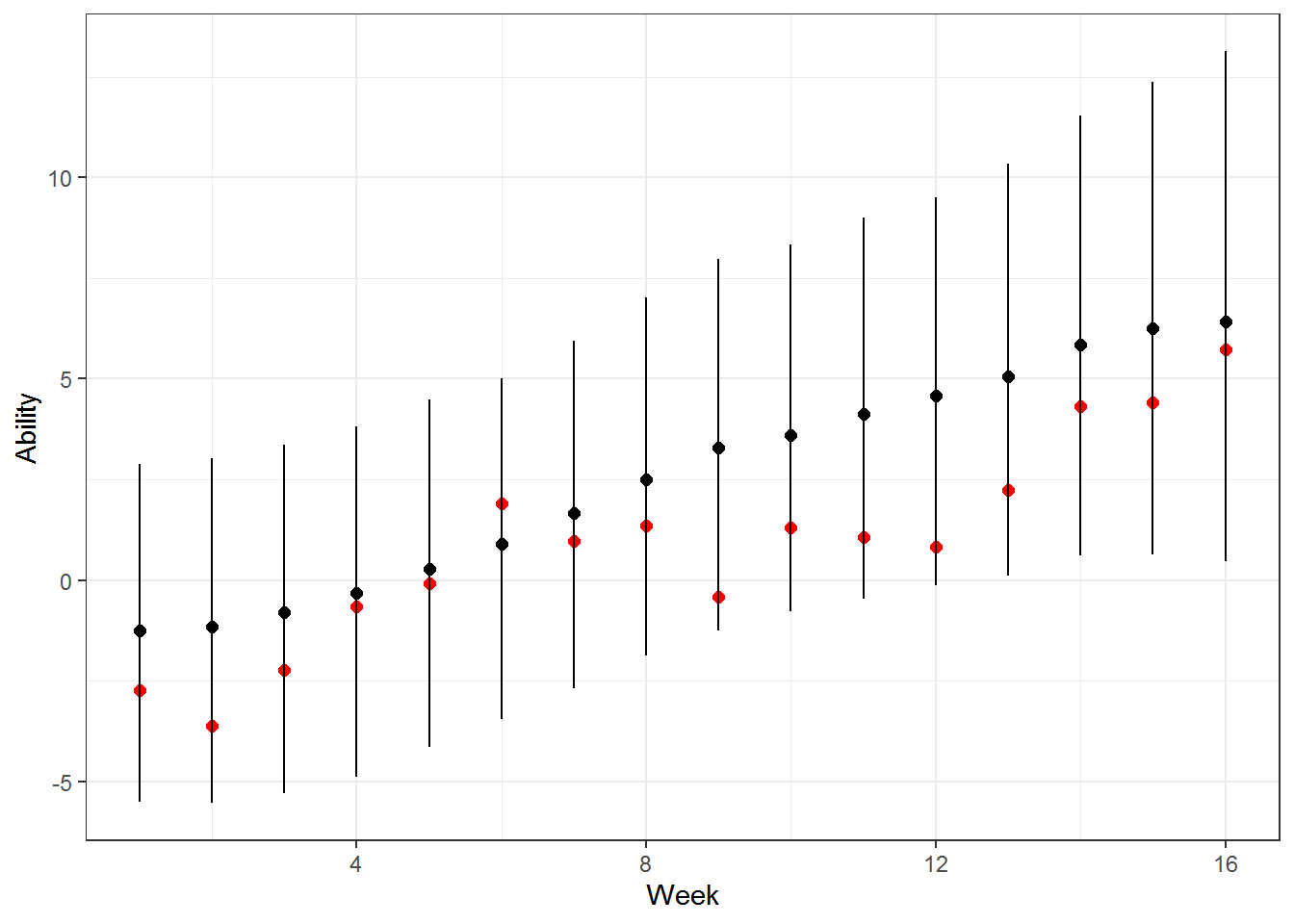
Why would team 1 be overrated at the end of the year? Their end of year results were really good!
filter(games, team_1 == 1 | team_2 == 1) %>%
  mutate(team_1_margin = if_else(team_1 == 1, score_diff, score_diff * -1)) %>%
  ggplot(aes(x = week, y = team_1_margin)) +
  geom_point() +
  geom_line() +
  xlab('Week') +
  ylab('Team 1 Margin of Victory')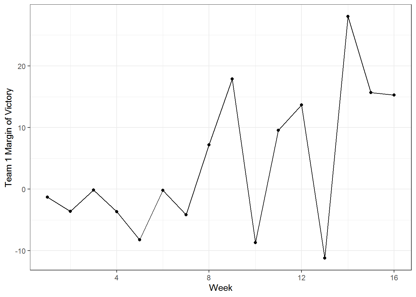
Concluding Thoughts
This is an extremely basic model to track changes in ability but that has a ton of useful applications. You can pretty easily extend this to include multiple indicators or build in different distributions on the state shocks.