I’ve been interested in getting better with purrr’s map functions and have always wanted to get my hands dirty with the Spotify API so this post has a little bit of both. We’ll use the wonderful spotifyr package to take a look at trends in which NFL players are hot topics of conversation on top Fantasy Football podcasts.
The first step was to identify a list of podcasts and pull their information. Based on some lists of the most popular podcasts and some personal domain knowledge we settled on the following:
- Fantasy Footballers
- The Ringer Fantasy Football Show
- CBS fantasy football today
- Fantasypros
- Fantasy Focus Football
- Late Round Podcast
- Establish the Run
- The Audible
- Yahoo Fantasy Football Forecast
- Rotowire
- PFF Fantasy
- The Underdog Football Show
The first step was to pull show descriptions from the last 50 episodes of each show. This is made very easy with the get_show_episides() funciton from spotifyr. To clean everything and we’ll define a function and used map_dfr to apply that function for each show and return a data frame with show id, release date, and the show’s text description for each episode. This left 582 total episodes.
library(nflfastR)
library(spotifyr)
library(tidyverse)
library(purrr)
library(plotly)
library(ggpubr)

pull_descriptions <- function(id){
  show <- spotifyr::get_show_episodes(id, limit = 50)
  df <- data.frame(id = show$id, description = show$description, release_date = show$release_date)
  df$release_date <- lubridate::ymd(df$release_date)
  return(df)
}

ids <- c("5RaNsb5sKEBleahQa4MVC5",
         "0XLPhMzcKmxoNziHkVkYpR",
         "2fEvGGxwXqSM8xuSNgxjFR",
         "1YM5ymt3vWVfdHzVAEzq2w",
         "55toF30GeLKhJYGr3JPQpG",
         "3sfbS4uuJNJtUTdnBG1KkI",
         "0gzBznDnd0yGIJ1hcv2NTW",
         "70E33T64jsqzqr9V0L9CFr",
         "0wf5ZBFRJnMSwIEgzhO2MQ",
         "3yJGYiR71iW2U5oyMG3jE6",
         "5Cph8h96Td7qaxFBxPADc9",
         "4k37aIxrGzggMOIvYrWBQb")

df <- map_dfr(ids, pull_descriptions)
Next, we want to find which players are being talked about. We can pull an up-to-date list of player names from the nflfastr package using the fast_scraper_roster function.
players <- fast_scraper_roster(2021) %>%
  filter(position %in% c('QB','RB','WR','TE'))
We want to identify every player mentioned in the episode’s description so we’ll create another function and use purrr to apply that function to each podcast episode. The function will return a data frame with a row for each player matched on a given day so if the show description has four player matches the function will return 4 rows.
get_matched_players <- function(show, date, description, player_vec){
  matches <- stringr::str_match(description, player_vec)
  matches <- matches[!is.na(matches)]
  if (length(matches) > 0){
    return_df <- data.frame(id = show, release_date = date, player = matches)
    return(return_df)
    }
}

player_matches <- pmap_dfr(.l = list(df$id, df$release_date, df$description),
                           .f = get_matched_players,
                           player_vec = players$full_name)

filter(player_matches, id == '6SlmIU5Vfn0j0T3K5LiPJp' & release_date == '2021-06-08')
## id release_date player
## 1 6SlmIU5Vfn0j0T3K5LiPJp 2021-06-08 Calvin Ridley
## 2 6SlmIU5Vfn0j0T3K5LiPJp 2021-06-08 Ryan Tannehill
## 3 6SlmIU5Vfn0j0T3K5LiPJp 2021-06-08 Julio Jones
## 4 6SlmIU5Vfn0j0T3K5LiPJp 2021-06-08 A.J. BrownAt this point we have all of our matched players but we’ll want to do a little more data manipulation. The plot below shows the number of podcasts episodes released and a couple of issues present themselves immediately. First, this data is very noisy day-to-day as there are certain days of the week where podcasts tend to come out. Next, there are seasonality effects where shows tend to release fewer episodes immediately after a season ends and pick up as the season nears.
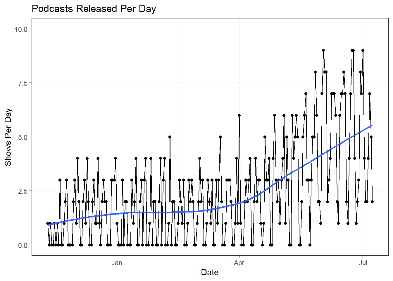
To deal with the day-to-day variation we’re going to calculate rolling averages by player and date, counting the total number of mentions in the two weeks leading up to a given date. To deal with the fact that there are more shows (and therefore more player mentions) as we get closer to the season we will define a metric, mention share, that is the rolling average of the player’s mentions at a given date divided by the rolling average of total player mentions at that same date. This will ensure that we adjust for the podcasting environment (new industry term that I’m trademarking right now) and treat mentions in July differently than mentions in March.
Before calculating rolling averages we want to make sure there is an entry for each player and date combination. The three data frames in the block below are counting player mentions by day, total mentions by day, and a rolling average of total mentions over a 14 day period.
full_mat <- expand.grid(seq(min(df$release_date), max(df$release_date), by = 1),
                        unique(player_matches$player))
full_mat <- data.frame(full_mat)
names(full_mat) <- c('release_date','player')

player_mentions_by_day <- full_mat %>%
  left_join(player_matches, by = c('release_date','player')) %>%
  mutate(mentioned = if_else(is.na(id), 0, 1)) %>%
  group_by(release_date, player) %>%
  summarise(n_mentions = sum(mentioned)) %>%
  ungroup()

player_mentions <- full_mat %>%
  left_join(player_matches, by = c('release_date','player')) %>%
  mutate(mentioned = if_else(is.na(id), 0, 1)) %>%
  group_by(player) %>%
  summarise(player_mentions_total = sum(mentioned)) %>%
  ungroup()


total_mentions_by_day <- player_mentions_by_day %>%
  group_by(release_date) %>%
  summarise(total_mentions = sum(n_mentions)) %>%
  ungroup() %>%
  mutate(rolling_total_mentions = zoo::rollsum(total_mentions,
                                               align = 'right',
                                               k = 14, na.pad = T)
         )
Player rolling averages weren’t playing nicely inside of dplyr so we’ll use yet another function and apply over each player in the data, returning a data frame with each player’s 14 day rolling average. At that point we can join our two rolling average data frames and divide the player rolling average by the total rolling average to get our mention share metric.
split_roll <- function(player_name, df){
  dat <- filter(df, player == player_name) %>%
    mutate(rolling_player_mentions = zoo::rollsum(n_mentions, align = 'right', k = 14, na.pad = T))
  return(dat)
}

rolling_player_mentions <- map_dfr(.x = unique(player_mentions_by_day$player),
                                   .f = split_roll,
                                   df = player_mentions_by_day)

final_dat <- rolling_player_mentions %>%
  left_join(total_mentions_by_day, by = 'release_date') %>%
  filter(release_date > '2021-01-01') %>%
  mutate(mention_share = rolling_player_mentions/rolling_total_mentions)
Visuals
At this point we have our data and can start to make some fun plots! Aaron Rodgers was in the news a ton this offseason and we can track exactly how the fantasy podcast world responded. We see a big uptick in mentions immediately after Packers were eliminated from the playoffs and Rodgers made some cryptic comments about play calling as well as big uptick in mentions around the draft in late April when some reporters started discussing him wanting to leave Green Bay.
We can also look at how the focus has changed on different players at different points in the offseason. Below we’re going to pull the 10 most mentioned running backs and plot their mention share across time. We see rookie running backs like Najee Harris, Travis Etienne, and Javonte Williams getting a lot of attention immediately after being drafted and falling back down to earth over the course of May.
rbs <- players %>%
  filter(position == 'RB') %>%
  select(full_name, position) %>%
  inner_join(player_mentions, by = c('full_name' = 'player')) %>%
  arrange(desc(player_mentions_total)) %>%
  slice(1:10)

rb_mentions <- final_dat %>%
  inner_join(rbs, by = c('player' = 'full_name'))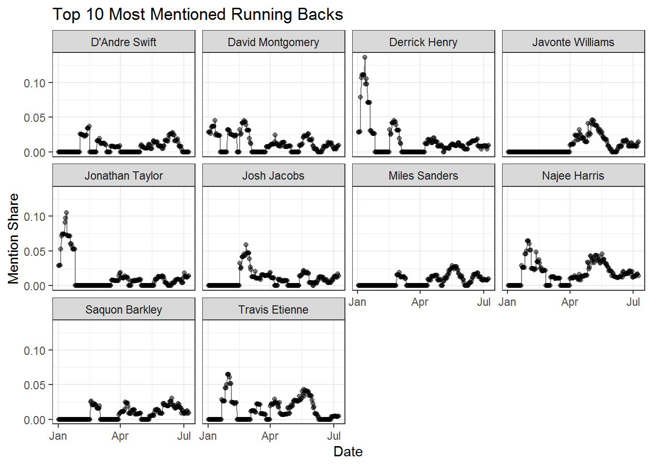
Next
I can think of a couple potential uses for information like this if any intrepid readers work in these areas:
- You host a fantasy football podcast and want to know who the industry is discussing
- This may be an indicator of future player value. Perhaps today’s heavily discussed players today are under/overdrafted in the future
- You are an Aaron Rodgers superfan and need to keep track of everything being said about him